CS7641 - Machine Learning - Unsupervised Learning
- Lecture Videos: https://omscs.gatech.edu/cs-7641-machine-learning-course-videos
- Books:
- Tom M. Mitchell. "Machine Learning." McGraw-Hill, 1997. (http://www.cs.cmu.edu/~tom/mlbook.html)
- Wasserman, L. (2004). All of Statistics: A Concise Course in Statistical Inference. New York: Springer. (https://www.stat.cmu.edu/~larry/all-of-statistics/)
- George's Notes (https://teapowered.dev/assets/ml-notes.pdf)
UL1: Randomized Optimization
Optimization Algorithm
- Input space $X$
- Objective function: Function that maps $x$ to a score $R$
- Score is also called fitness, objective, etc.
- Goal: Find $x^* \in X$ subject to $f(x^*)=max_x f(x)$
- Find $x^*$ so that $f(x^*)$ returns as close as possible to the maximum possible value.
Uses:
- Process control (systems optimization)
- Route finding
- Root finding (of a function)
- Neural networks (x as weights, minimize error)
- Decision Trees (x as order of nodes, minimize error)
Quiz: Optimize Me
Given $x=\{1, \ldots, 100\}$, optimize the following functions
- $f(x)= (x\mod6)^2 \mod 7 - \sin(x)$
- $f(x)= -x^4 + 1000x^3 - 20x^2 + 4x - 6$
ANSWER:
- Q1: 11
- Q2: 750
"""Solve Quiz via Generate & Test"""
from math import sin
import matplotlib.pyplot as plt
def fn_1(x: int):
return (x % 6) ** 2 % 7 - sin(x)
def fn_2(x: int):
return -(x**4) + 1000 * x**3 - 20 * x**2 + 4 * x - 6
# Generate and Test to get max value of f(x)
fn_1_x = list(range(1, 100))
fn_2_x = list(range(-500, 1000)) # Subtitute R with large range
result_fn_1 = tuple(fn_1(i) for i in fn_1_x)
result_fn_2 = tuple(fn_2(i) for i in fn_2_x)
fn_1_max = max(result_fn_1)
fn_2_max = max(result_fn_2)
fn_1_max_x = result_fn_1.index(fn_1_max) + 1
fn_2_max_x = result_fn_2.index(fn_2_max) - 500 # Offset index by -500
# Print maximum x and its value
print("Q1 - index:", fn_1_max_x, "value:", fn_1_max)
print("Q2 - index:", fn_2_max_x, "value:", fn_2_max)
# Plot it
fig, ax = plt.subplots(1, 2, figsize=(10, 3))
ax[0].plot(fn_1_x, result_fn_1)
ax[0].set_title("Function 1 and Optimal x")
ax[0].axvline(x=fn_1_max_x, color="r")
ax[1].plot(fn_2_x, result_fn_2, color="red")
ax[1].set_title("Function 2 and Optimal x")
ax[1].axvline(x=fn_2_max_x, color="b");

Takeaway: We can use methods below, but each have caveats:
- Generate & Test (see code) - Works with small input space or complex function.
- Calculus - Assumes function has a derivative and solvable = 0
- Newton's method (gradient ascent) - Function has derivative, but expects single optimum (can get s tuck in local optima)
These assumptions don't hold if:
- Big input space (G&T)
- Complex function (Calculus, Newton)
- No derivative (or hard to find) (Calculus, Newton)
- Possibly many local optima (Newton)
The solution, is to use Random Optimization
Hill Climbing (Non-random)
Algorithm (steepest ascent hill climbing):
- Find neighbor with the highest function value.
- If neighbor is above current value, move to the new point.
- Otherwise, stop (either local/global optima)

Quiz: Guess my word/bits

Takeaways: Well behaved problem. This problem has only 1 optima.
Random Restart Hill Climbing
Algorithm
Once local optimum reached, try again starting from a randomly chosen x.
- Multiple tries to find a good starting place.
- Not much more computationally expensive (constant factor).
Issues
If the range of input space that reaches global optimum is narrow (ie green zone in image), then there is high chance that we will only random restart at point where it reaches the local optima (ie yellow zone)

Quiz: Random Hill Climbing Eval
This is a complicated answer, watch video for full info: https://www.youtube.com/watch?v=Ts9vLVxyqdY

Takeaway: The success of random hillclimbing depends a lot on the size of the attraction base (area that points toward global optima). If it is narrow, it won't do as much better than trying every point in $X$.
Simulated Annealing
Motivation
Idea: "Don't alaways improve (exploit) - sometimes you need to search (explore) with the hope of finding something even better".
- Hill climbing can be considered 100% exploiting, which is more likely to leading to local optima. Kind of like "believing too much" in your data, which relates to overfitting.
Algorithm
From CMU notes:
The algorithm is basically hill-climbing except instead of picking the best move, it picks a random move. If the selected move improves the solution, then it is always accepted. Otherwise, the algorithm makes the move anyway with some probability less than 1. The probability decreases exponentially with the “badness” of the move, which is the amount deltaE by which the solution is worsened.
Simulated annealing is typically used in discrete, but very large, configuration spaces, such as the set of possible orders of cities in the Traveling Salesman problem and in VLSI routing.

Key Ideas:
- If $f(x_t)$ is greater than $f(x)$, we just accept it and move to $x_t$.
- If T (temperature) goes to infinity, like hill climbing. If T goes to zero, like random walk. Why?
- Hill Climbing: If low T, numerator becomes big. $\frac{x_t - x}{T}$ goes to infinity and its inverse of $e$ goes to zero. Zero means we reject $x_t$.
- Random Walk: If high T, numerator doesn't matter. $\frac{x_t - x}{T}$ goes to zero, meaning $e^0$. Its inverse is $\frac{1}{e^0}=1$. 1 means we accept $x_t$.
- Metallurgy analogy: "High temperature, molecules bounce around (random). Cold temperature, molecules stay put (hill climb)".
- How to apply? Decrease $T$ slowly over time.
Properties of Simulated Annealing
- Probability of ending at x is most likely at areas of high fitness $f(x)$
- As $T$ goes down, the formula acts like a max, putting all the probability mass on $x^*$
- As $T$ goes up, the distribution becomes more random.
- Formula is simlar to the Boltzmann Distribution
Genetic Algorithms
Reference:
- Mitchell, Ch.9 "Genetic Algorithms" p.249
Motivation
Terminology:
- Population: Group of individual search points.
- Mutation: Local search of each individual along their neighborhoods.
- Crossover - Takes different points of individuals and combines them together to find a more optimal location.
- Generations - Iterations of improvement across the population.

Takeaways:
- Like random hill climbing but done with parallel computing.
- Crossover - Population shares information with each other.
Algorithm
- $P_0$ : Initialize population of size $K$
- Repeat until converged:
- Compute fitness over all individuals in population $x \in P_t$
- Select "most fit" individuals. How?
- "Truncation Selection" - Top half of those that returned best value given $f(x)$. Weighed towards exploitation.
- "Roulette Wheel" - Select individuals at random, but give x's with higher scores a higher probability of being selected. Weighted towards exploration.
- Pair up most fit individuals and create new point via crossover/mutation. New offspring replaces "least fit" individuals
Crossover Example

Takeaways:
- 1-point crossover and inductive bias: If split at index, locality of bits matter (bits closer together, stay together). Bias because location of information might matter.
- Uniform crossover: Exact same distribution over each pair, locality doesn't matter.
Summary: RO pt.1
- Randomized Optimization: Random steps, start in random places. Useful if no gradient pointing the way.
- Types: Hill climbing, Hill climbing + random restarts.
- Simulated annealing: Temperature, captures probability distribution.
- Genetic algorithms: Population, crossover, parallel random hill climbing
- Overall, these algorithms are memoryless.
MIMIC
Reference: De Bonet, Isbell, Viola, "MIMIC: Finding Optima by Estimating Probability Densties", 1997
Motivation
- Other algos were memoryless, and no structure (just points) were being communicated.
- Unclear what probability distribution we are dealing with.
How? Directly model a probability distribution and succesfully refine this model over time. This then conveys the structure the search space and its best points.

Algorithm
- Generate samples from distribution at time step $t$: $P(x)^{\theta_t}$
- ie, "Population"
- Set $\theta_{t+1}$ to the $n$th percentile (ie. 50th percentile, etc)
- Like Genetic Algorithm, choose those that are "best fits"
- Retain only those samples (subject to $f(x) \geq \theta_{t+1}$)
- ie. "Most fit"
- Estimate $P(x)^{\theta_{t+1}}$
- ie. "Structure"
- Repeat until convergence
- Ideally we will move from $\theta_{min}$ to $\theta_{max}$
Challenges:
- Assumes we can estimate $P(x)^{\theta_{t+1}}$.
- Assumes diff between $P^\theta$ and $P^{\theta_\epsilon}$ should be close, ie. current sample would contain samples from the next distribution we're looking for.
- The higher $P^\theta$ becomes, it becomes harder to represent the distribution of input space.
Estimating Distributions

* Example of joint probability distribution (ref):
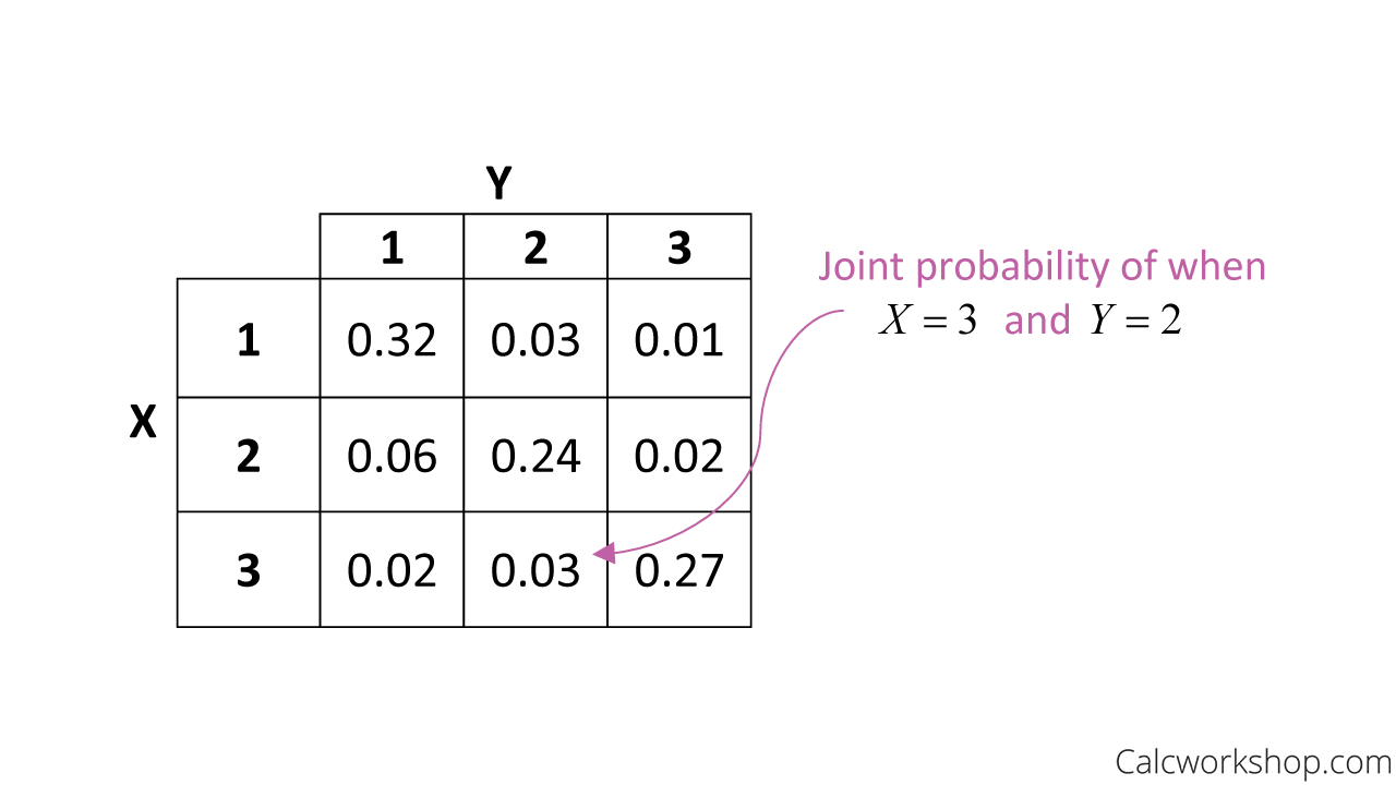
Finding Dependency Trees
NOTE: I got lost on the math. Revisit this lecture to refresh: https://www.youtube.com/watch?v=R-Mf9-tKC5o.

Takeaway: The best dependency tree we can find is the one that minimizes all of the entropy for each of the features, given the product of its parents.
- Looking at it another way - To find the best dependency tree, is to maximize mutual information between every feature and its parent (last equation). Best DT is the one that captures dependencies the best.
- Use Prim's algorithm to find the maximum spanning tree.
Quiz: Probability distributions
Motivation: MIMIC doesn't care about the probability distribution, the user must pick the best one.
Q: Given 3 problems and 3 probability distributions you might use, see which distribution works best for each problem.
A:

Takeaway: Each probability distributions represent a structure, ie each $x$'s relationship to each other.
Practical Matters
- MIMIC does well with structure
- ie. Does well when optimal values depend only on the structure (see quiz slide for context).
- RHC, SA gets confused when 2+ optima exist but their values look very different from one another.
- Must represent probability distribution of everything.
- Local optima is still a problem.
- You get probability theory for free.
- Time Complexity: Much less iterations, but each iteration is more expensive compared to SA, RHC.
- MIMIC works best when cost of evaluating your fitness function is high (e.g. simulation, involving human eval)
UL2: Clustering
The overall structure of this section of the course is to look at UL algorithms that are each designed to solve different problems.
Basic Clustering Problem:
- Given: Set of objects $X$ and inter-object distances $D(x,y)=D(y,x)$ where $x,y \in X$,
- Output: Partition, ie. partition function defined for distance D for object x $P_D(x) = P_D(y)$ is the same if both x and y are in the same cluster.
- Example: All in one cluster $\forall_x P_D(x)=1$, each x is its own cluster $\forall_x P_D(x)=x$
Single Linkage Clustering
Algorithm
- Consider each object a cluster ($n$ objects)
- Define intercluster distance as the distance between closest two points in the two clusters
- Merge two closest clusters
- Repeat $n-k$ times to make $k$ clusters.
Quiz: Time Complexity
Q: Given $n$ points (objects) and $k$ clusters, what is its running time?
- A: $O(n^3)$ - Inherently quadratic ($O(n^2)$) since it needs to consider distance across all nodes. And additionally must repeakt $k$ times ($\frac{n}{2}$)
Quiz: Unexpected Clusters

K-means Clustering
Algorithm
- Pick $k$ centers at random.
- While not converged (ie. no more data points change clusters):
- Each center "claims" its closest points
- Recompute the centers by averaging the clustered points (ie. find "centroids")
K-means in Euclidean Space

K-means as Optimization
Reference: Notes from ISYE6501


K-means Properties
- Each iteration is polynomial $O(Kn)$
- Finite (exponential) iterations $O(K^n)$
- Error monotonically decreases (if ties broken consistently)
- Can get stuck if initial K cluster centers are close to each other.
- Workaround: Random restarts, like hill climbing - or choosing K centers far enough away from each other.
Soft Clustering
TODO: I don't understand what is meant by "selecting K Gaussians" here, it seems related to the Gaussian Process but I don't understand what that is either.

Motivation: If one $x$ is exactly between 2 clusters, sometimes included in partition A, then partition B. Can we put ambiguous examples into both clusters?
Algorithm
Assume the data was generated by the following method:
- Select one of $k$ gaussians (w/ fixed known variance) uniformly
- Sample a data point $x_i$ from that Gaussian
- Repeat $n$ times.
- Idea: If $n$ is bigger than $k$ then we'll see some points that comes from the same Gaussian, and if those Gaussians are well separated (ie. different means) they'll look like clusters.
Task: Find a hypothesis of means $h = \{ \mu_1 \ldots \mu_k\}$ that maximize the probability of the data (Maximum Likelihood).
Application
From George's Notes:
$$ x = \{x, z_1, z_2 \ldots z_i\} $$Single Max Likelihood Gaussian: Suppose k = 1 for the simplest possible case. What Gaussian maximizes the likelihood of some collection of points? Conveniently (and intuitively), it’s simply the Gaussian with μ set to the mean of the points!
Extending to Many Ks: With k possible sources for each point, we’ll introduce hidden variables for each point that represent which cluster they came from. They’re hidden because, obviously, we don’t know them: if we knew that information we wouldn’t be trying to cluster them. Now each point x is actually coupled with the probabilities of coming from the clusters:
Expectation Maximization
Algorithm
Idea: Move back and forth calculating 2 probabilistic distributions: Expectation, and Maximization, ie. adjusting the cluster probabilities zi and the chosen mean μ
Terminology:
- $E[z_{ij}]$: Likelihood that data $i$ comes from cluster $j$.

Application
From George's Notes:

EM Properties
- Finds higher and higher likelihoods over each iteration (ie. "monotonically non-decreasing"), but amount can get smaller and smaller.
- Theoretically does not guarantee convergence (like k-means), but practically it does.
- Can get stuck at local optima, but get around it by random restart.
- Works with any distribution (ie. not just Gaussian), given that expectation and maximization are solvable.
Clustering Properties
Richness: For any given set of data assigned to clusters $C$, there is some distance matrix $D$ that causes your clustering algo $P_D$ to produce that clustering.
- $\forall c, \exists D : P_D = C$
- "Given data points, allow any kind of clustering output"
Scale-invariance: Scaling distances doesn't change the clustering (x100, different units, etc).
- $\forall D, \forall k > D : P_D = P_{kD}$
Consistency: Shrinking distance of points within a cluster AND increasing distance between clusters doesn't change the clustering.
- $P_D = P_D`$
Impossibility Theorem

Answer:
- We sacrifice richness because we're limiting the number of allowable clusters.
- We sacrifice scale-invariance because we can change distance metric $\theta$. Scaling the points by θ would result in each point belonging to its own cluster.
- We sacrifice consistency because $W$ can change the maximum. By shrinking points within a cluster, it changes maximum distance and thus causes a different clustering.
Impossibility Theorem by Kleinberg:
No clustering schema can achieve all three of: Richness, scale invariance and consistency.
Summary: Clustering
Types:
- K-Means
- Single Linkage Clustering (terminates fast)
- Expectation Maximization (soft clusters, other 2 are "hard" clusters)
UL3: Feature Selection
Motivations:
- Knowledge Discovery - Good for interpretability and insight of your data.
- Curse of Dimensionality - The amount of data required grows exponentially as more features are added $2^N$.
Quiz: Given a set of $N$ features and a function $f$ that returns a score, how hard is the problem of choosing the best subset of $N$ ($m$)?

Feature Selection Algorithms

Filtering
Definition: Search combinations of features using a heuristic, pass it to learner (L)
Pros/Cons: It is fast, but you don't get feedback from the learner. It is ignoring the learning problem.
Technique:
- Decision Trees are in its own way a filtering algo. It uses a metric (information gain, variance, entropy, etc) to decide which feature to split on. You can actually use a DT separately to get important features, then use just those feature for a different ML algo (KNN, NN, etc).
- It's also useful to only use features that are independent, dependent variables doesn't offer utility given feature it depends on.
Wrapping
Definition: Search combinations of features and for each combo, get feedback from the learner.
Pros/Cons: It is much slower ($2^N$), but since it gets information from the learner over each iteration, it accounts for model bias and learning.
Technique:
- Optimization: We can use approaches directly from randomized optimization algorithms if we treat the learner’s result as a fitness function
- Search: Can use forward search or backwards search to find best set of features (see notes from ISYE650-Forward-Selection)).
Quiz: Feature Selection of DT / NN
Q: What's the smallest set of features sufficient to net zero training error, given a DT and NN?

Relevance vs Usefulness
Relevance is a way to measure how useful a feature is to learn a problem.
- Feature $x_i$ is strongly relevant if removing it degrades the Bayes Optimal Classifier (BOC).
- Feature $x_i$ is weakly relevant if:
- Not strongly relevant
- $\exists$ subset of features $S$ such that adding $x_i$ to $S$ improves BOC
- Otherwise, feature $x_i$ is irrelevant.
Usefulness: A feature’s usefulness is measured by its effect on a particular predictor rather than on the Bayes’ optimal classifier
UL4: Feature Transformation
What is it?: Feature transformation is the pre-processing of features into a smaller, more compact feature set that still retains as much relevant and useful information as the original.
- Transform features into another: $x\sim F^N=F^M$
- New set is smaller than original: $M<N$
- Project original data $X$ into matrix $P$ to get new set of features which are linear combinations of old features: $P^T_X$
Motivation: Example - Information Retrieval
Problem: Given a database and a search term, we want to return the most relevant set of documents. What features do we use? We can use words, but there are many words which can lead to the curse of dimensionality. Words can also be ambiguous (e.g. "book" as a noun vs verb).
Solution: We can use feature transformation to group relevant words together, which ends up creating a more compact feature set.

Principal Components Analysis
Reference:
Principal Components Analysis is a technique in which we can project features into a ranked set of new "component" features, which are determined by the amount of variance the component explains.
The first PC of a feature set represents the direction of maximum variance. Subsequent PCs are orthogonal to each other, and importantly explain the next direction of maximal variance.
Eigenvectors are a set of vectors used to transform a source matrix $X$ into a transformed matrix $\lambda$, which are called eigenvalues. One can move from $X$ to $\lambda$ by multiplying either matrix with the eigenvector. Given matrix $X$, each principal component is the linear transformation of X by a ranked set of eigenvectors (eg. $Xv_1 \ldots Xv_n$ are principal components)

Independent Components Analysis
Independent Components Analysis is slightly different from PCA, in that instead of finding vectors that maximizes variance (and correlation), it aims to maximize independence. This means that if feature set $X$ is transformed into $Y$ via ICA, each of the features $Y_i$ share minimal/zero mutual information between one another while still retaining all of the original information.
- Applications: In the lecture, it covers the "cocktail party" problem, ie blind source separation.
From Georges Notes:
From a high level, given some features {x1,x2,...}, ICA aims to find new features {y1,y2,...} such that $y_i \bot y_j$ and $I(yi,yj) = 0$ (that is, the pairs of vectors are mutually independent and share minimal mutual information). It also tries to maximize the mutual information between the $x_i$s and $y_j$s.

Mechanics (Cocktail Party Example)

- Given N microphones, we align them and take samples, ie a spectrogram at a fast sample rate. In the image, each column represents a sample.
- ICA attempts to take each sample of N microphones and find a projection that would create a new feature space that maximizes statistical independence of each (ie microphone).
- Yet, we still have high mutual information between original source $X$ and transformed features $Y$, so that we aren't losing any information.
- IMPORTANT: ICA is heavily dependent on this assumption of the underlying hidden variables being independent. If the data doesn't have independent features, ICA will not be able to fit it.
ICA vs PCA Quiz


Takeaways:
- PCA/ICA returns different features given different datasets (faces, natural scenes, documents)
- PCA tends to focus on the average (ie. brightness, average face) since it tries to explain global variance.
- ICA tends to focus on specific features (ie. nose, eyes, edges, topics) since its focus is on independence.
Alternative Algos
- Random Components Analysis: Projects original data with a random vector. This surprisingly works well when used for classification purposes, because it reduces the number of dimensions thus avoiding the curse of dimensionality. And even when randomly projecting, new features still pick up correlations along the way.
- Big advantange over PCA: FAST. Very simple, cheap and it works!
- Linear Discriminant Analysis: Finds projection that discriminates based on the label, very much like supervised learning. Pretty similar to SVM.
UL5: Information Theory
Motivation: In general, every input/output vector (in ML context) can be thought of as a probability density function*. IT is a mathematical framework that lets us compare these density functions to ask questions like (from George's notes):
- Which of our $x_i$'s will give us the most information about the output?
- Are these input feature vectors similar? This is called mutual information.
- Does this feature have any information? This is called entropy.
* Mathematical function that describes the probability of an event occurring
Entropy
Entropy is the measure of uncertainty associated with a random variable.
- More predictable sequence = send less data. Less predictable sequence = send more data.


Formula
Entropy in general is expressed as follows, where:
- $P(s)$ is the probability of the symbol occurring, and
- $\log_2 P(s)$ is the size of the symbol.
Mutual Information
Mutual Information gives us information about the relationship between variables (ie. given rain, P of thunder). We can measure this in a few ways:
Joint Entropy measures randomness given a set of variables: * ($h$ represents entropy)
$$ h(X,Y) = -\sum_{x \in X, y \in Y} P(x,y) \log_2 P(x,y) $$Conditional Entropy measures the randomness of one variable given another variable:
$$ h(Y | x) = -\sum_{y \in Y} P(x,y) \log_2 P(Y|x) $$- If two variables are independent, we can ignore the prior: $h(Y|x) = h(Y)$. This means the joint entropy is represented as the sum of both entropy $H(X,Y) = H(X) + H(Y)$.
Mutual Information (MI) measures the mutual dependence of random variables. It measures the amount of information both X and Y share. High MI means X and Y are highly dependent, low MI means they are independent.
$$ I(x,Y) = h(Y) - h(Y|x) $$Quiz Pt.1
(TODO: This was tricky, revisit entropy calculation)
Answer the probability of the following, where A and B are 2 independent coins with P(0.5)
- $P(A,B)$ = 0.25 (Product of A & B)
- $P(A|B)$ = 0.5 (Independent so prior doesn't matter)
- $H(A)$ = 1
- $-\sum P(A) log P(A)$
-2*(0.25*math.log(0.25,2))(python)
- $H(B)$ = 1
- $H(A,B)$ = 2
- $-\sum P(A,B) log P(A,B)$
-4*(0.25*math.log(0.25,2))(python)
- $H(A|B)$ = 1
- $-\sum P(A,B) log P(A|B)$
-4*(0.25*math.log(0.5)(python)
- $I(A,B)$ = 0
- $H(A) - H(A|B)$
- If independent, no mutual independent info between them!
Quiz Pt.2
Answer the probability of the following, where A and B are 2 dependent coins with P(0.5)
- $P(A,B)$ = 0.5 (Can be either both heads or both tails, 2 out of 4 conditions)
- $P(A|B)$ = 1
- $P(A|B) = \frac{P(A,B}{B}$
0.5/0.5
- $H(A)$ = 1
- $-\sum P(A) log P(A)$
-2*(0.25*math.log(0.25,2))(python)
- $H(B)$ = 1
- $H(A,B)$ = 2
- $-\sum P(A,B) log P(A,B)$
-2*(0.5*math.log(0.5,2))(python)
- $H(A|B)$ = 0
- $-\sum P(A,B) log P(A|B)$
-2*(0.5*math.log(1,2)(python)
- $I(A,B)$ = 1
- $H(A) - H(A|B)$
- Since coins are dependent now, mutual information shows that random variable A shares information with random variable B.
Kullback-Leibler Divergence (KL Divergence)
KL Divergence measures the distance between two distributions. Mutual information is special case of KL divergence.
$$ D_{KL} (p || q) = \int P(x) log_2 \frac{P(p)x}{P(q)x} dx $$- Always non-negative
- Only zero if p = q
- Non-symmetric measure: KL divergence from distribution A to distribution B is not necessarily the same as the KL divergence from distribution B to distribution A.
Significance: In SL our goal is to model data $X$ to a distribution which is unknown $p(x)$. We can sample this data to get a known distribution $q(x)$. We can use KL divergence as a substitute for the least square formula for fitting.